WGCNA

workflowr

• Summary
• Checks
• Past versions

Last updated: 2023-08-29

Checks: 7 0

Knit directory: DEPDC5_D62_Analysis/

This reproducible R Markdown analysis was created with workflowr (version 1.7.0). The Checks tab describes the reproducibility checks that were applied when the results were created. The Past versions tab lists the development history.

---

R Markdown file: up-to-date

Great! Since the R Markdown file has been committed to the Git repository, you know the exact version of the code that produced these results.

Environment: empty

Great job! The global environment was empty. Objects defined in the global environment can affect the analysis in your R Markdown file in unknown ways. For reproduciblity it’s best to always run the code in an empty environment.

Seed: set.seed(20220808)

The command set.seed(20220808) was run prior to running the code in the R Markdown file. Setting a seed ensures that any results that rely on randomness, e.g. subsampling or permutations, are reproducible.

Session information: recorded

Great job! Recording the operating system, R version, and package versions is critical for reproducibility.

Cache: none

Nice! There were no cached chunks for this analysis, so you can be confident that you successfully produced the results during this run.

File paths: relative

Great job! Using relative paths to the files within your workflowr project makes it easier to run your code on other machines.

Repository version: 9dd12f1

Great! You are using Git for version control. Tracking code development and connecting the code version to the results is critical for reproducibility.

The results in this page were generated with repository version 9dd12f1. See the Past versions tab to see a history of the changes made to the R Markdown and HTML files.

Note that you need to be careful to ensure that all relevant files for the analysis have been committed to Git prior to generating the results (you can use wflow_publish or wflow_git_commit). workflowr only checks the R Markdown file, but you know if there are other scripts or data files that it depends on. Below is the status of the Git repository when the results were generated:

Ignored files:
    Ignored:    .Rproj.user/
    Ignored:    output/D62_dds_matrix.RData
    Ignored:    output/D62_mdsplots.RData

Note that any generated files, e.g. HTML, png, CSS, etc., are not included in this status report because it is ok for generated content to have uncommitted changes.

---

These are the previous versions of the repository in which changes were made to the R Markdown (analysis/04_D62_WGCNA.Rmd) and HTML (docs/04_D62_WGCNA.html) files. If you’ve configured a remote Git repository (see ?wflow_git_remote), click on the hyperlinks in the table below to view the files as they were in that past version.

File	Version	Author	Date	Message
html	9dd12f1	achiocch	2023-08-29	wflow_publish(c("./analysis/", "code/"), all = T)
html	20e7956	achiocch	2023-07-31	Build site.
Rmd	6cbb9a0	achiocch	2023-07-25	plots fro publication added
Rmd	c1f2468	achiocch	2022-10-11	sets the installation procedure in the readme
html	a7c5f57	achiocch	2022-10-10	fix intaller
Rmd	3f72d3a	Andreas Geburtig-Chiocchetti	2022-08-26	full analysis pre manuscript version
html	3f72d3a	Andreas Geburtig-Chiocchetti	2022-08-26	full analysis pre manuscript version
html	ddade00	achiocch	2022-08-19	Build site.
Rmd	4bd303c	achiocch	2022-08-19	wflow_publish(c("./*"))
Rmd	974c39d	achiocch	2022-08-18	wflow_publish(c("./*"))
html	974c39d	achiocch	2022-08-18	wflow_publish(c("./*"))
html	dc78d32	Andreas Geburtig-Chiocchetti	2022-08-09	full analysis pre manuscript version
Rmd	f249225	achiocch	2022-08-08	adds data and code

---

WGCNA

soft thresholding

allowWGCNAThreads()

Allowing multi-threading with up to 16 threads.

dds2 = DESeq(ddsMat)

using pre-existing size factors

estimating dispersions

found already estimated dispersions, replacing these

gene-wise dispersion estimates

mean-dispersion relationship

final dispersion estimates

fitting model and testing

vsd = getVarianceStabilizedData(dds2)

WGCNA_matrix <- t(log2(vsd+1)) #Need to transform for further calculations

#s = abs(bicor(WGCNA_matrix)) #biweight mid-correlation
powers = c(c(1:10), seq(from = 12, to=20, by=2))
sft = pickSoftThreshold(WGCNA_matrix, powerVector = powers, verbose = 5)

pickSoftThreshold: will use block size 3258.
 pickSoftThreshold: calculating connectivity for given powers...
   ..working on genes 1 through 3258 of 13731
   ..working on genes 3259 through 6516 of 13731
   ..working on genes 6517 through 9774 of 13731
   ..working on genes 9775 through 13032 of 13731
   ..working on genes 13033 through 13731 of 13731
   Power SFT.R.sq  slope truncated.R.sq mean.k. median.k. max.k.
1      1    0.234 -0.862          0.909 2910.00  2.82e+03   4940
2      2    0.827 -1.350          0.978  983.00  8.49e+02   2630
3      3    0.935 -1.470          0.984  425.00  3.07e+02   1700
4      4    0.949 -1.490          0.971  216.00  1.24e+02   1230
5      5    0.949 -1.480          0.963  124.00  5.48e+01    945
6      6    0.946 -1.450          0.956   77.20  2.56e+01    759
7      7    0.938 -1.420          0.948   51.50  1.26e+01    627
8      8    0.943 -1.390          0.955   36.10  6.42e+00    530
9      9    0.937 -1.360          0.952   26.40  3.40e+00    456
10    10    0.943 -1.330          0.959   19.90  1.84e+00    397
11    12    0.938 -1.300          0.963   12.20  5.84e-01    311
12    14    0.937 -1.270          0.969    8.08  1.99e-01    251
13    16    0.939 -1.250          0.974    5.62  7.26e-02    207
14    18    0.932 -1.250          0.970    4.06  2.83e-02    174
15    20    0.931 -1.250          0.973    3.03  1.15e-02    148

par(mfrow = c(1,2))
cex1 = 0.9;
plot(sft$fitIndices[,1], -sign(sft$fitIndices[,3])*sft$fitIndices[,2],
     xlab="Soft Threshold (power)",ylab="Scale Free Topology Model Fit, signed R^2",
     type="n", main = paste("Scale independence"));
text(sft$fitIndices[,1], -sign(sft$fitIndices[,3])*sft$fitIndices[,2],
     labels=powers,cex=cex1,col="red");
abline(h=0.80,col="red")

plot(sft$fitIndices[,1], sft$fitIndices[,5],xlab="Soft Threshold (power)",ylab="Mean Connectivity", type="n",main = paste("Mean connectivity"))
text(sft$fitIndices[,1], sft$fitIndices[,5], labels=powers, cex=cex1,col="red")

Identify Gene Modules

softPower = 6;

# The point where the curve flattens
#calclute the adjacency matrix

if(reanalyze | !file.exists(paste0(output,"/D62_WGCNA_adj_TOM.RData"))){
  #adj= adjacency(WGCNA_matrix,type = "unsigned", power = softPower);
  
  #Converting adjacency matrix into To so that the noise could be reduced
  TOM=TOMsimilarityFromExpr(WGCNA_matrix,networkType = "unsigned", 
                            TOMType = "unsigned", power = softPower);
  save(list = c(
    #"adj", 
    "TOM"), file=paste0(output,"/D62_WGCNA_adj_TOM.RData"))
  
} else {
  load(paste0(output,"/D62_WGCNA_adj_TOM.RData"))
}

TOM calculation: adjacency..
..will not use multithreading.
 Fraction of slow calculations: 0.000000
..connectivity..
..matrix multiplication (system BLAS)..
..normalization..
..done.

SubGeneNames<-colnames(WGCNA_matrix)

colnames(TOM) =rownames(TOM) =SubGeneNames
dissTOM=1-TOM
diag(dissTOM) = 0

#hierarchical clustering
geneTree = flashClust(as.dist(dissTOM),method="average");

#plot the resulting clustering tree (dendrogram)
# plot(geneTree, xlab="", sub="",cex=0.3, main="Module clustering prio to merging");

#Set the minimum module size
minModuleSize = 50;

#Module identification using dynamic tree cut
dynamicMods = cutreeDynamic(dendro = geneTree, 
                            distM = dissTOM, 
                            cutHeight = 0.998,
                            minClusterSize = minModuleSize,
                            deepSplit=2, 
                            pamRespectsDendro = T)

 ..done.

#the following command gives the module labels and the size of each module. Lable 0 is reserved for unassigned genes
#table(dynamicMods)

#Plot the module assignment under the dendrogram; note: The grey color is reserved for unassigned genes
dynamicColors = labels2colors(dynamicMods)
table(dynamicColors)

dynamicColors
    black      blue     brown     green      grey       red turquoise    yellow 
      276      2306      1716      1024       404       658      6000      1347 

plotDendroAndColors(geneTree, dynamicColors, "Dynamic Tree Cut", 
                    dendroLabels = FALSE, hang = 0.03, 
                    addGuide = TRUE, 
                    guideHang = 0.05, 
                    main = "Gene dendrogram and module colors")

diag(dissTOM) = NA;

#Visualize the Tom plot. Raise the dissimilarity matrix to the power of 4 to bring out the module structure
TOMplot(dissTOM^4, geneTree, as.character(dynamicColors), main="weighted distance of Topological overlap Matrix")

Module eigengenes

Identify and Merge correlated modules

#calculate eigengenes
MEList = moduleEigengenes(WGCNA_matrix, colors = dynamicColors)
MEs = MEList$eigengenes 

plotEigengeneNetworks(MEs, "Eigengenes_before_merging", 
                      marDendro = c(0,4,1,2), marHeatmap = c(3,4,1,2))

MEList_new = mergeCloseModules(WGCNA_matrix, colors = dynamicColors, MEs = MEs, cutHeight = 0.05)

 mergeCloseModules: Merging modules whose distance is less than 0.05
   Calculating new MEs...

plotEigengeneNetworks(MEList_new$newMEs, "Eigengenes_after_merging", 
                      marDendro = c(0,4,1,2), marHeatmap = c(3,4,1,2))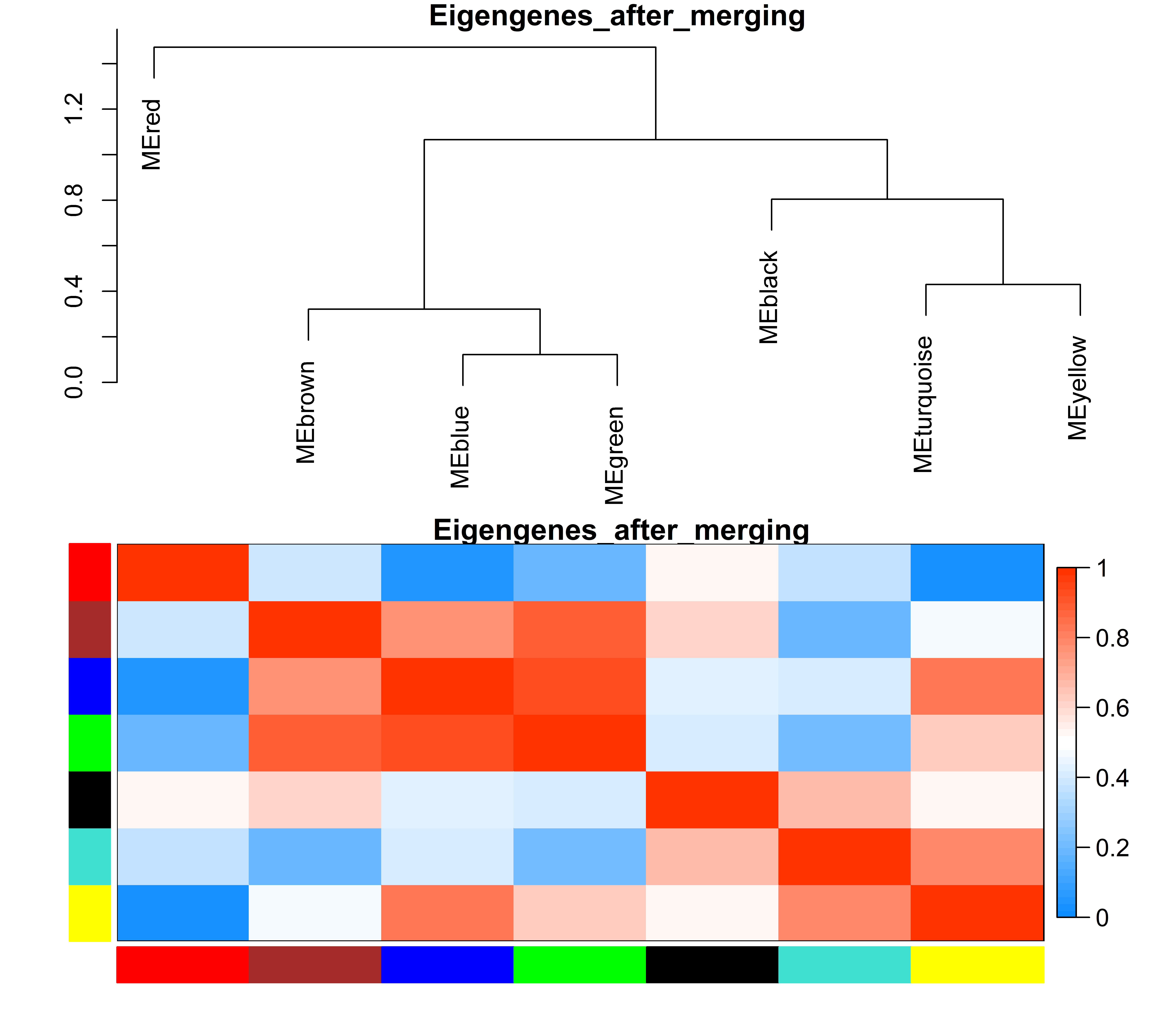

MEs = MEList_new$newMEs

coldata_all = colData(ddsMat) %>% as.data.frame() %>% 
  select(-grep("ME", colnames(colData(ddsMat)), value = T)) %>% 
  cbind(MEs[colnames(ddsMat),]) %>% DataFrame()

colData(ddsMat) = coldata_all

colors_new = MEList_new$colors

mcols(ddsMat) = cbind(mcols(ddsMat)%>% as.data.frame() %>% select(-contains("cluster")), data.frame(cluster=colors_new)) %>% DataFrame()

Heatmaps MEs

#colors for plotting heatmap
colors <- rev(colorRampPalette(brewer.pal(9, "Spectral"))(255))


gRNAcol = Dark8[c(1:nlevels(SampleInfo$gRNA))+nlevels(SampleInfo$CellLine)]
names(gRNAcol) = levels(SampleInfo$gRNA)

diffcol = brewer.pal(3,"Set1")[1:nlevels(SampleInfo$DIFF)]
names(diffcol) = levels(SampleInfo$DIFF)

rapacol = brewer.pal(3,"Set2")[1:nlevels(SampleInfo$RAPA)]
names(rapacol) = levels(SampleInfo$RAPA)

clustcol = gplots::col2hex(unique(as.character(mcols(ddsMat)$cluster)))
names(clustcol) = unique(as.character(mcols(ddsMat)$cluster))

rownames(WGCNA_matrix)=SampleInfo[rownames(WGCNA_matrix), "label_rep"]

ann_colors = list(
  DIFF = diffcol, 
  RAPA = rapacol,
  gRNA = gRNAcol,
  cluster = clustcol)

idx=order(SampleInfo$gRNA, SampleInfo$DIFF,SampleInfo$RAPA)
WGCNA_matrix_sorted=WGCNA_matrix[SampleInfo$label_rep[idx], order(colors_new)]

collabels = SampleInfo[idx,c("gRNA","DIFF", "RAPA")] %>%  
  mutate_all(as.character) %>% as.data.frame()

rownames(collabels)=SampleInfo$label_rep[idx]

genlabels = data.frame(cluster = as.character(colors_new)[order(colors_new)])
rownames(genlabels) = colnames(WGCNA_matrix_sorted)


MElabels = data.frame(cluster = gsub("ME", "",colnames(MEs)))
rownames(MElabels) = colnames(MEs)

clustcol = gplots::col2hex(unique(as.character(MElabels$cluster)))
names(clustcol) = as.character(MElabels$cluster)

ann_colors = list(
  DIFF = diffcol, 
  RAPA = rapacol,
  gRNA = gRNAcol,
  cluster = clustcol)

rownames(MEs) = SampleInfo[rownames(MEs),"label_rep"]

pheatmap(t(MEs[idx,]),
         border_color = NA, 
         annotation_row = MElabels,
         annotation_col = collabels,
         cluster_cols = F,
         show_rownames = F, show_colnames = F,
         clustering_method = "ward.D2",
         annotation_colors = ann_colors,
         scale="row",
         breaks  = seq(-2, 2,length.out=255),
         col = colors, 
         main = "eigengene values")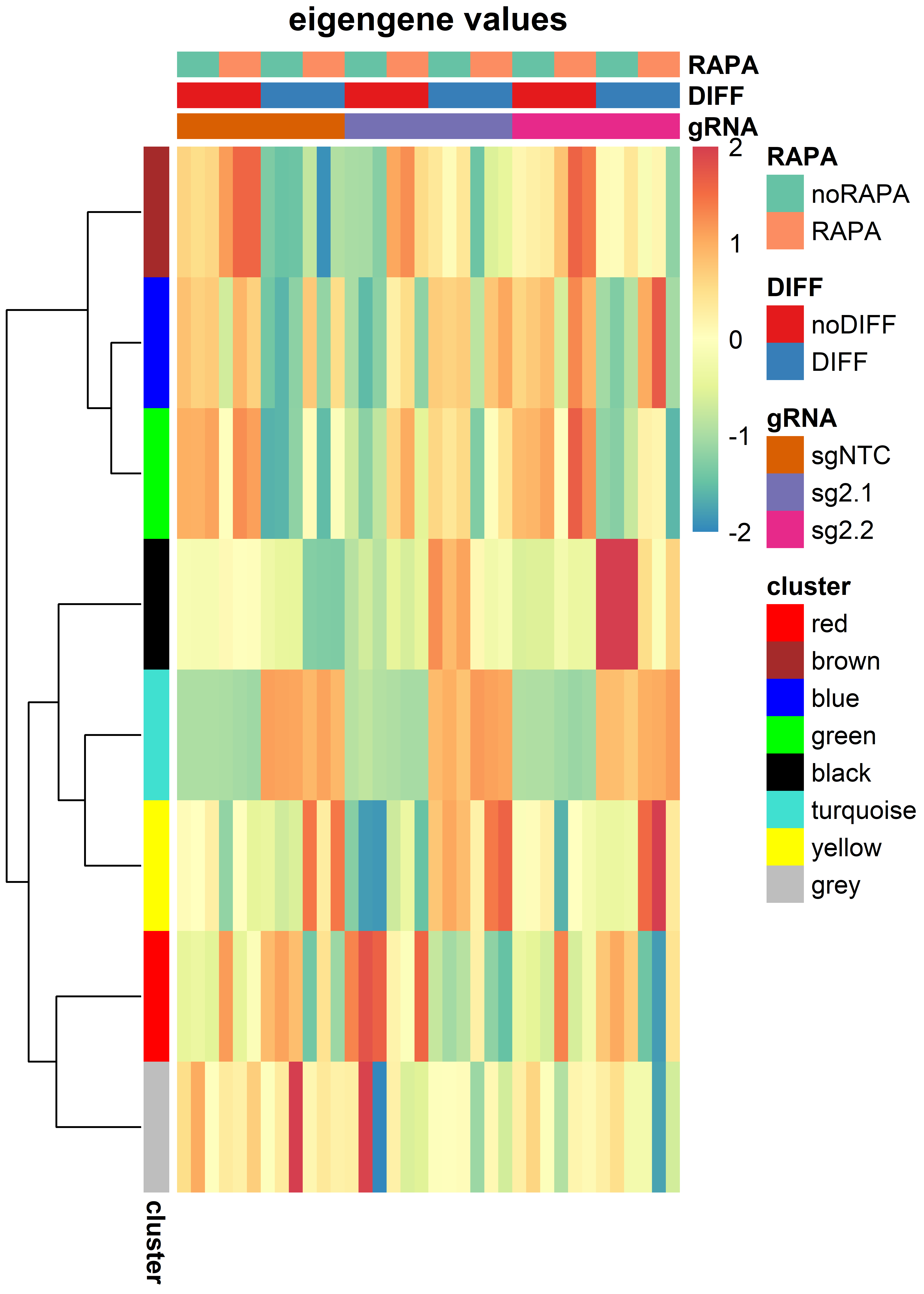

SampleInfo = as.data.frame(colData(ddsMat))
MEMat = SampleInfo[,grep("ME", colnames(SampleInfo))]



## helper functions#test differences
testit=function(Dataset, samples = Set, 
                depvar){
  data = Dataset[samples,]
  res=list()
  for(i in grep("ME", colnames(data), value = T)){
    res[[i]]=lm(as.formula(paste0(i,"~1+",depvar)), data)
  }
  return(res)
}



# extract coefficents
getcoefff=function(x){
  res = summary(x)$coefficients[2,]
  return(res)
}

# comparisonME
comparisonME = function(SampleInfo, Set, target){
  LMlist=testit(Dataset = SampleInfo, samples = Set, depvar=target)
  coeff = as.data.frame(lapply(LMlist, getcoefff) %>% do.call(rbind, .))
  coeff$padj = p.adjust(coeff$`Pr(>|t|)`, "bonferroni")
  return(coeff)}

## comparisons against noRAPA NTC
Rapamycin=c("noRAPA", "RAPA")
Differentiation=c("noDIFF", "DIFF")
Type_sgRNA<-c("sg2.1","sg2.2")
target="KO"

r = Rapamycin[1]
d = Differentiation[1]
Tp = Type_sgRNA[[1]]


# no random effects included 
for(r in Rapamycin){
  Rapafilter = SampleInfo$RAPA %in% r
  for(d in Differentiation){
    Difffilter = SampleInfo$DIFF %in% d
    for(Tp in Type_sgRNA){
      sgRNAfilter = SampleInfo$gRNA %in% Tp
      vs_label=paste0(c("sgNTC", Tp), sep="", collapse="_")
        Set = rownames(SampleInfo)[Rapafilter&Difffilter&
                                     sgRNAfilter]
        Set = c(Set, rownames(SampleInfo)[SampleInfo$RAPA == "noRAPA" & Difffilter&
                                     SampleInfo$gRNA == "sgNTC"])
        lab = paste("restabWGCNA", "D62_NTCnoRAPA", vs_label, d,r, sep="_")
        assign(lab, comparisonME(SampleInfo, Set, target))
    }
  }
}



# comparison agains RAPANTC
Rapamycin=c("noRAPA", "RAPA")
Differentiation=c("noDIFF", "DIFF")
Type_sgRNA<-list(c("sgNTC","sg2.1"),c("sgNTC", "sg2.2"))
target="KO"

# comparison agains RAPANTC
for(r in Rapamycin){
  Rapafilter = SampleInfo$RAPA %in% r
  for(d in Differentiation){
    Difffilter = SampleInfo$DIFF %in% d
    for(Tp in Type_sgRNA){
      sgRNAfilter = SampleInfo$gRNA %in% Tp
      vs_label=paste0(Tp, sep="", collapse="_")
        Set = rownames(SampleInfo)[Rapafilter&Difffilter&
                                     sgRNAfilter]
        lab = paste("restabWGCNA", "D62_NTCwRAPA", vs_label, d,r, sep="_")
        assign(lab, comparisonME(SampleInfo, Set, target))
    }
  }
}

comparisons= apropos("restabWGCNA_D62")
save(list = comparisons, file = paste0(home,"/output/D62_ResTabs_WGCNA.RData"))

mypval=0.05
MEIds = rownames(get(apropos("restabWGCNA")[1]))

getWGCNAoutputs = function(targetline="D62",targetdiff,
                           targetrapa, refset="NTCnoRAPA", plotset=T){
  
    if(refset=="NTCnoRAPA"){
    samplesincl=SampleInfo$DIFF==targetdiff &
      SampleInfo$RAPA==targetrapa &  
      SampleInfo$KO == "KO"
    samplesincl = samplesincl | (SampleInfo$DIFF==targetdiff &
      SampleInfo$RAPA=="noRAPA" &  
      SampleInfo$KO == "WT")} else {
        samplesincl=SampleInfo$DIFF==targetdiff &
      SampleInfo$RAPA==targetrapa
      }
  
  
  pvalrep=  get(paste0("restabWGCNA_", 
                       targetline,"_",refset, "_sgNTC_sg2.1_", 
                       targetdiff, "_" , 
                       targetrapa))$padj<=mypval &
    get(paste0("restabWGCNA_", 
               targetline, "_",refset, "_sgNTC_sg2.2_", 
               targetdiff, "_" , 
               targetrapa))$padj<=mypval
  
  betarep = apply(cbind(get(paste0("restabWGCNA_", 
                                   targetline, "_",refset, "_sgNTC_sg2.1_", 
                                   targetdiff, "_" , 
                                   targetrapa))$Estimate,
                        get(paste0("restabWGCNA_", 
                                   targetline, "_",refset, "_sgNTC_sg2.2_", 
                                   targetdiff, "_" , 
                                   targetrapa))$Estimate), 1,
                  samesign)
  
  idx=which(betarep & pvalrep)
  hits=MEIds[idx]
  
  
  restab=data.frame(
    Module = MEIds, 
    beta_2.1 = get(paste0("restabWGCNA_", 
                          targetline,"_",refset,  "_sgNTC_sg2.1_", 
                          targetdiff, "_" , 
                          targetrapa))$Estimate, 
    bonferroni_2.1 = get(paste0("restabWGCNA_", 
                                targetline, "_",refset, "_sgNTC_sg2.1_", 
                                targetdiff, "_" , 
                                targetrapa))$padj, 
    beta_2.2 = get(paste0("restabWGCNA_", 
                          targetline,"_",refset,  "_sgNTC_sg2.2_", 
                          targetdiff, "_" , 
                          targetrapa))$Estimate, 
    bonferroni_2.2 = get(paste0("restabWGCNA_", 
                                targetline, "_",refset, "_sgNTC_sg2.2_", 
                                targetdiff, "_" , 
                                targetrapa))$padj)
  
  print(restab)
  write.xlsx(restab, file=paste0(output, "/Restab_", 
                                 targetline,"_",refset, "_", 
                                 targetdiff, "_",
                                 targetrapa, ".xlsx"))
  SamplesSet=SampleInfo[samplesincl,] %>% select(all_of(hits))
  if(plotset){
  EigengenePlot(SamplesSet, SampleInfo, samplesincl)}
  
}

Eigengene plots all modules

EigengenePlot(data=SampleInfo[,grep("ME", colnames(SampleInfo))],
              Sampledata = SampleInfo, 
              samplesincl=rep(T, nrow(SampleInfo)))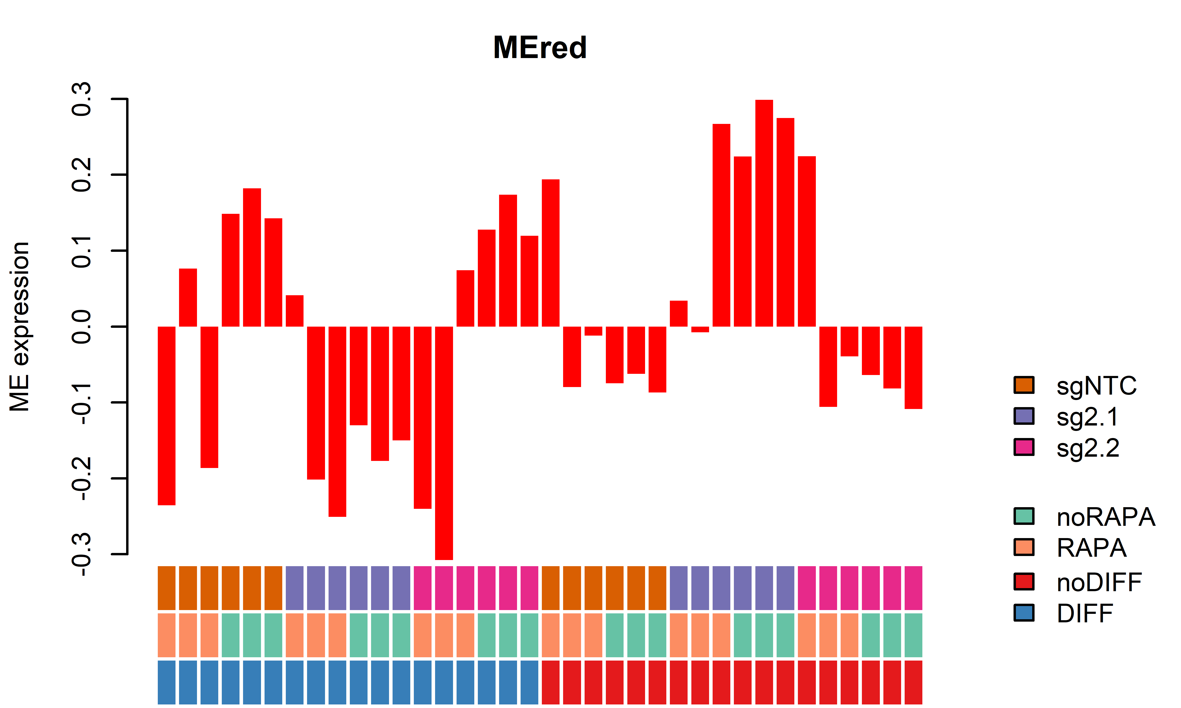

WGCNA module plots only D62

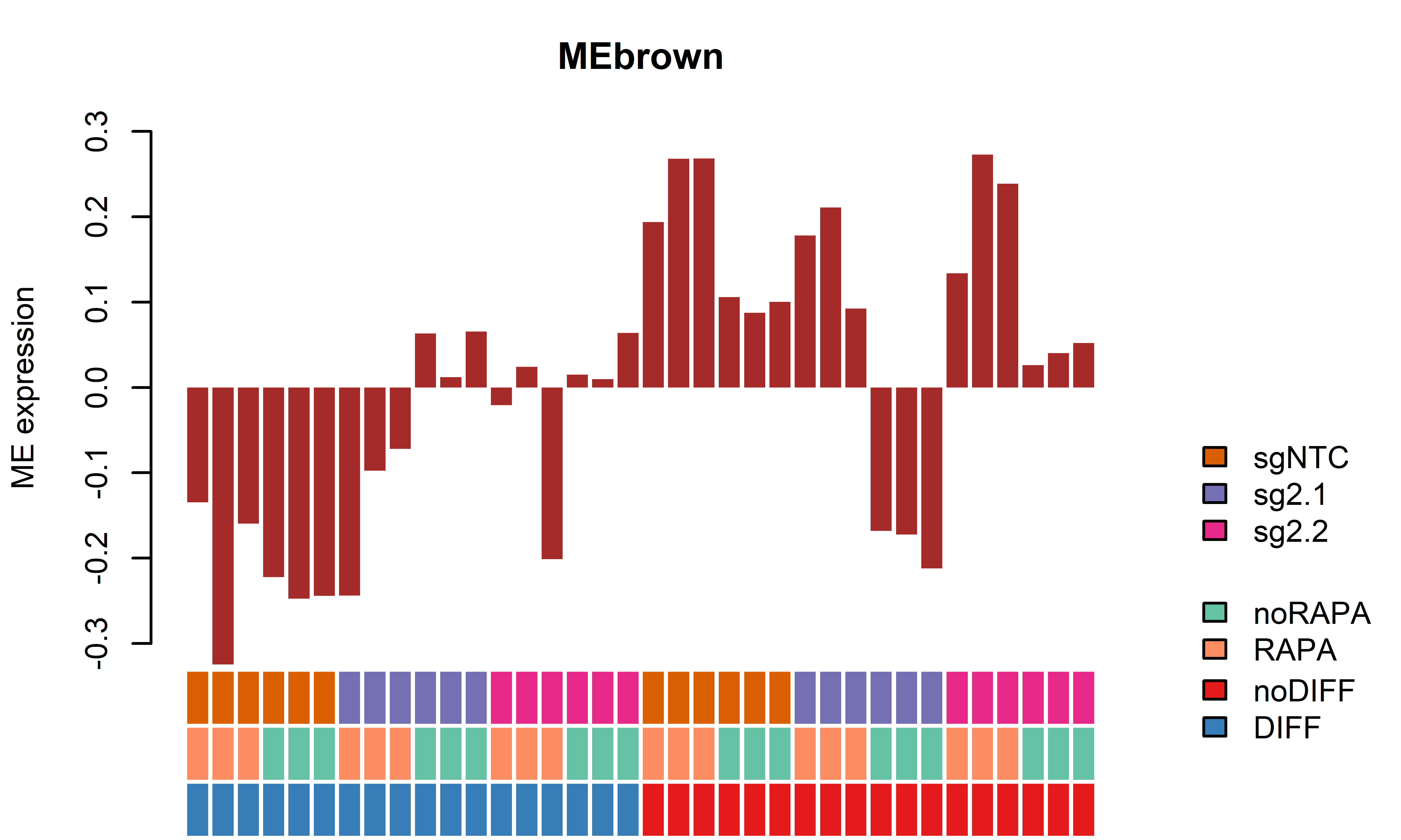
KO effect in noDIFF noRAPA

D62

getWGCNAoutputs(targetdiff = "noDIFF",targetrapa = "noRAPA", plotset = T)

       Module    beta_2.1 bonferroni_2.1     beta_2.2 bonferroni_2.2
1       MEred  0.34049833   0.0009947568 -0.009847209   1.000000e+00
2     MEbrown -0.28206000   0.0003735108 -0.058385040   2.518703e-02
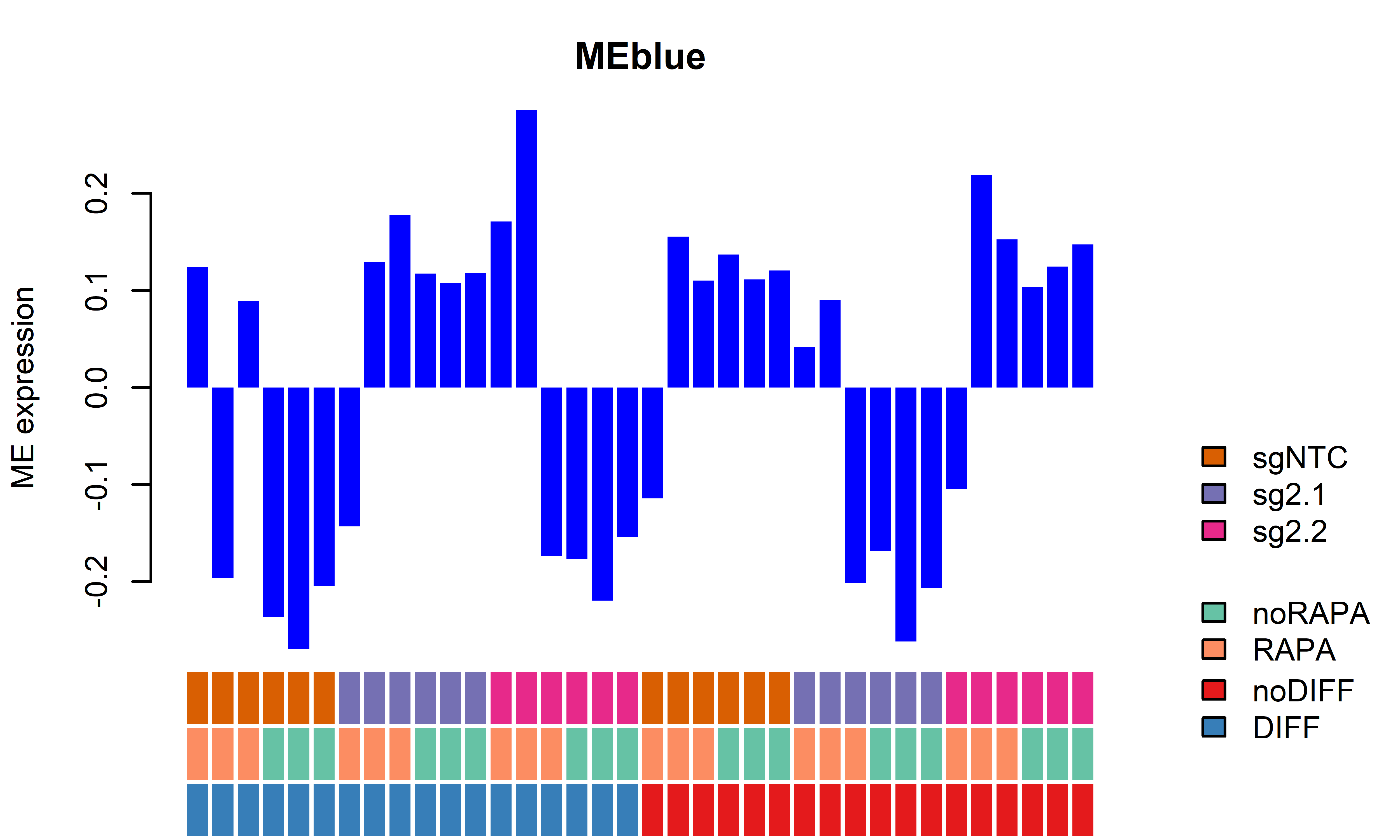
3      MEblue -0.33523842   0.0022606324  0.002375805   1.000000e+00
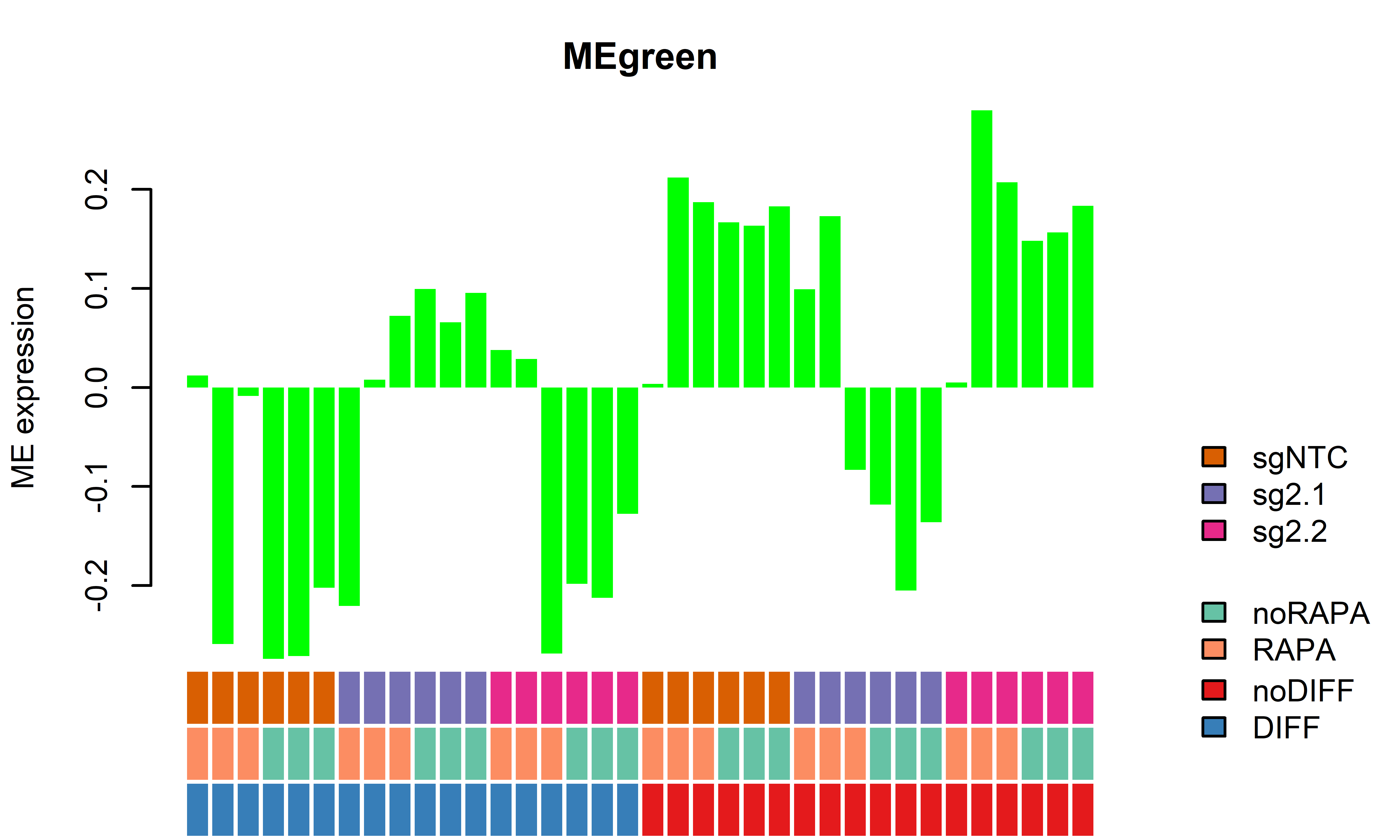
4     MEgreen -0.32410775   0.0022396816 -0.008367778   1.000000e+00
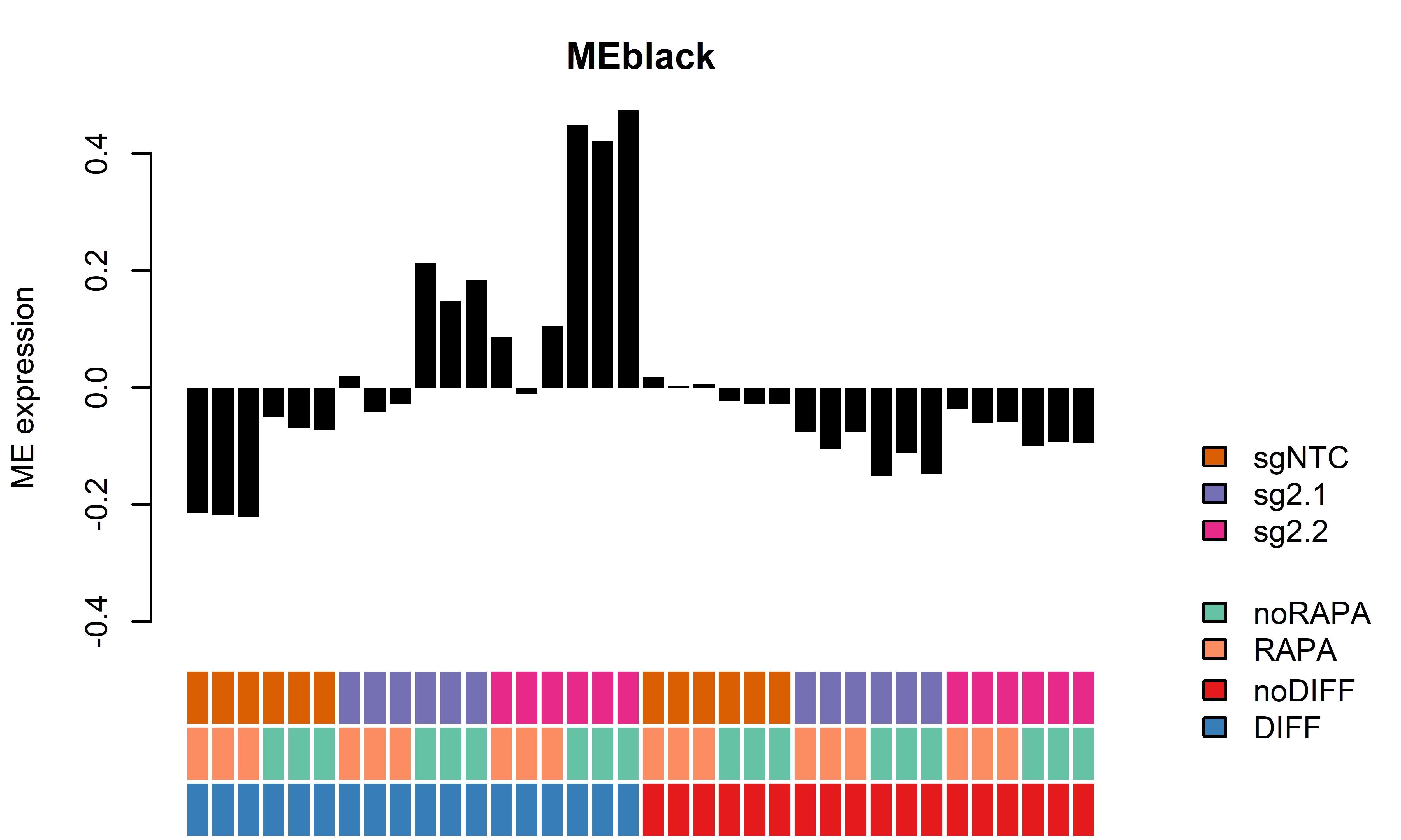
5     MEblack -0.11039767   0.0079997639 -0.069518536   7.682637e-05
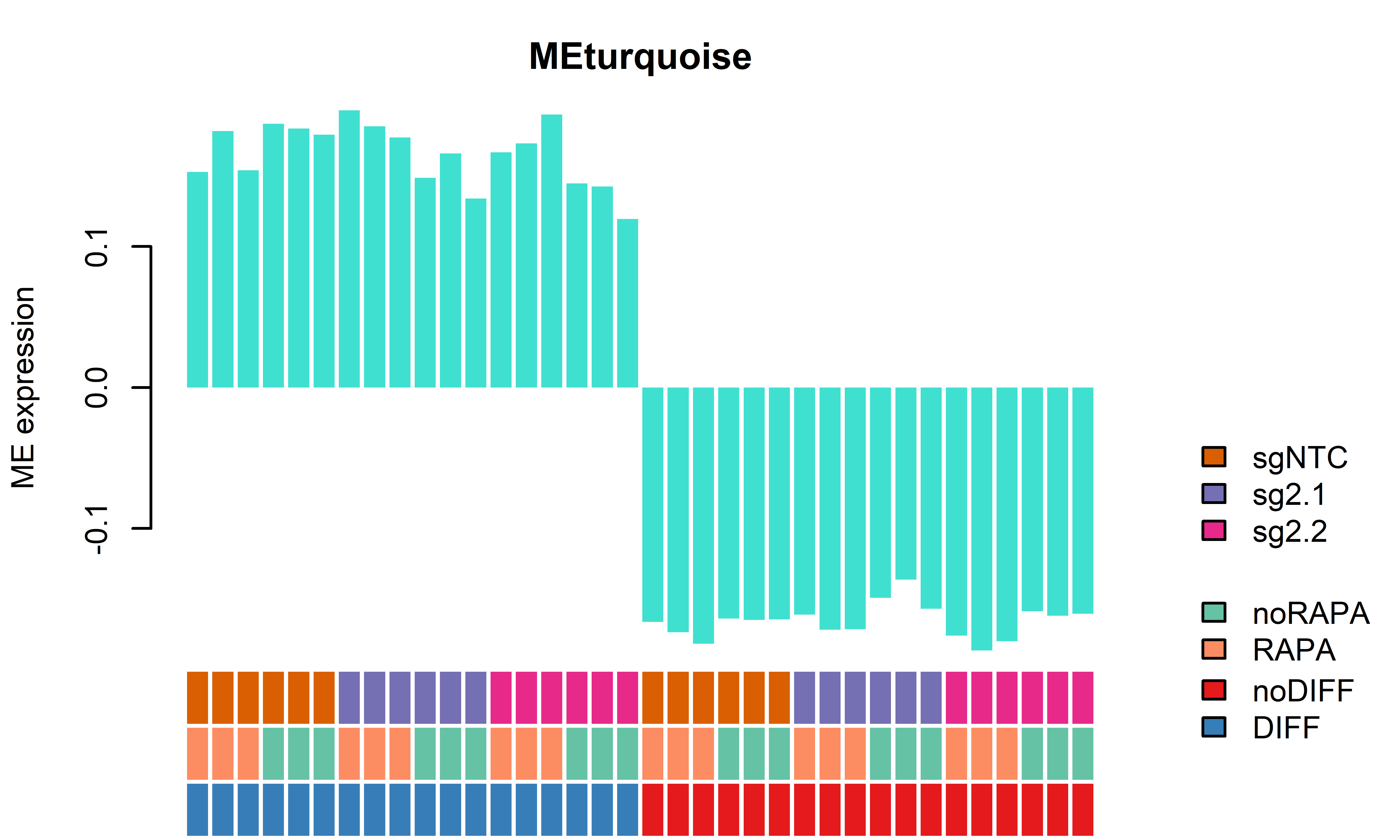
6 MEturquoise  0.01696263   0.3861421012  0.004109875   1.101362e-01
7    MEyellow -0.29617673   0.0084866670 -0.005792508   1.000000e+00
8      MEgrey -0.18704459   1.0000000000 -0.040649469   1.000000e+00

KO effect in DIFF noRAPA

D62

getWGCNAoutputs(targetdiff = "DIFF",targetrapa = "noRAPA", plotset = T)

       Module    beta_2.1 bonferroni_2.1    beta_2.2 bonferroni_2.2
1       MEred -0.31000479   0.0005785977 -0.01738949   1.000000e+00
2     MEbrown  0.28494983   0.0009531967  0.26751850   1.186855e-03
3      MEblue  0.35131310   0.0004080748  0.05345781   9.457238e-01
4     MEgreen  0.33612032   0.0016021205  0.06979599   9.492983e-01
5     MEblack  0.24588372   0.0018629558  0.51251646   5.187381e-05
6 MEturquoise -0.03377917   0.1895466925 -0.04773828   3.723205e-02
7    MEyellow  0.24513519   0.0018442002  0.03527412   5.519585e-01
8      MEgrey -0.14601285   1.0000000000 -0.11812970   1.000000e+00

KO effect in noDIFF RAPA

D62

getWGCNAoutputs(targetdiff = "noDIFF",targetrapa = "RAPA", refset = "NTCwRAPA" , plotset = T)

       Module     beta_2.1 bonferroni_2.1     beta_2.2 bonferroni_2.2
1       MEred  0.063701420    1.000000000 -0.007754679     1.00000000
2     MEbrown -0.082873602    1.000000000 -0.028123938     1.00000000
3      MEblue -0.073531605    1.000000000  0.038619733     1.00000000
4     MEgreen -0.071292095    1.000000000  0.029769245     1.00000000
5     MEblack -0.094069613    0.006916798 -0.060935174     0.02118051
6 MEturquoise  0.005791482    1.000000000 -0.006929335     1.00000000
7    MEyellow -0.050955126    1.000000000 -0.013454312     1.00000000
8      MEgrey -0.120824426    0.609904240 -0.107417138     1.00000000

getWGCNAoutputs(targetdiff = "noDIFF",targetrapa = "RAPA", refset = "NTCnoRAPA" , plotset = T)

       Module     beta_2.1 bonferroni_2.1     beta_2.2 bonferroni_2.2
1       MEred  0.172550699     0.91485849  0.101094599     1.00000000
2     MEbrown  0.062588843     1.00000000  0.117338508     0.39737331
3      MEblue -0.145985884     1.00000000 -0.033834546     1.00000000
4     MEgreen -0.108069293     1.00000000 -0.007007953     1.00000000
5     MEblack -0.058527235     0.03022928 -0.025392796     0.28882806
6 MEturquoise -0.003593694     1.00000000 -0.016314511     0.04912674
7    MEyellow -0.161668997     0.38875014 -0.124168183     1.00000000
8      MEgrey -0.137741921     0.84785240 -0.124334633     1.00000000

KO effect in DIFF RAPA

D62

getWGCNAoutputs(targetdiff = "DIFF",targetrapa = "RAPA", refset = "NTCwRAPA" , plotset = T)

       Module    beta_2.1 bonferroni_2.1    beta_2.2 bonferroni_2.2
1       MEred -0.02196168    1.000000000 -0.04280098     1.00000000
2     MEbrown  0.06846119    1.000000000  0.14037625     1.00000000
3      MEblue  0.04906314    1.000000000  0.08871593     1.00000000
4     MEgreen  0.03845811    1.000000000  0.01787810     1.00000000
5     MEblack  0.20084728    0.003557251  0.27884853     0.01207385
6 MEturquoise  0.02340289    0.799383362  0.01486376     1.00000000
7    MEyellow  0.00412049    1.000000000  0.04545928     1.00000000
8      MEgrey -0.13340904    0.743595737 -0.18919134     0.58800950

getWGCNAoutputs(targetdiff = "DIFF",targetrapa = "RAPA", refset = "NTCnoRAPA" , plotset = T)

       Module     beta_2.1 bonferroni_2.1     beta_2.2 bonferroni_2.2
1       MEred -0.294763402      0.2542855 -0.315602699      0.4472014
2     MEbrown  0.100193723      1.0000000  0.172108789      0.5446000
3      MEblue  0.291478418      0.3637644  0.331131204      0.6093049
4     MEgreen  0.202459592      0.7402675  0.181879584      1.0000000
5     MEblack  0.047129344      0.6176020  0.125130599      0.2148778
6 MEturquoise  0.003062091      1.0000000 -0.005477041      1.0000000
7    MEyellow  0.277153407      0.1630285  0.318492193      0.1866296
8      MEgrey -0.240546841      1.0000000 -0.296329138      0.9021750

KO additional Plots for better visulization

dataset=SampleInfo[,grep("brown|black", colnames(SampleInfo))]
idx=order(SampleInfo$RAPA, SampleInfo$gRNA)
SampleInfosort = SampleInfo[idx,]

EigengenePlot(data=dataset,
              Sampledata = SampleInfosort, 
              samplesincl=SampleInfosort$DIFF=="noDIFF")

EigengenePlot(data=dataset,
              Sampledata = SampleInfosort, 
              samplesincl=SampleInfosort$DIFF=="DIFF")

gene_univers = rownames(ddsMat)

Genes_of_interset = split(rownames(ddsMat), mcols(ddsMat)$cluster)

gostres = getGOresults(Genes_of_interset, gene_univers, evcodes = T)

toptab = gostres$result

write.xlsx(toptab, file = paste0(output,"/D62_GOresWGCNA.xlsx"), sheetName = "GO_enrichment")

for (module in names(Genes_of_interset)){
  idx = toptab$query==module & grepl("GO", toptab$source)
  if(!any(idx)){
    p = ggplot() + annotate("text", x = 4, y = 25, size=4, 
                            label = "no significant GO term") + 
      ggtitle(module)+theme_void()+
      theme(plot.title = element_text(hjust = 0.5))
  } else {
    p=GOplot(toptab[idx, ], 10, Title =module)
  }
  print(p)
}

Warning: Removed 10 rows containing missing values (`geom_point()`).

save(ddsMat, file=paste0(output,"/D62_dds_matrix.RData"))

Session information

sessionInfo()

R version 4.2.0 (2022-04-22 ucrt)
Platform: x86_64-w64-mingw32/x64 (64-bit)
Running under: Windows 10 x64 (build 19045)

Matrix products: default

locale:
[1] LC_COLLATE=German_Germany.utf8  LC_CTYPE=German_Germany.utf8   
[3] LC_MONETARY=German_Germany.utf8 LC_NUMERIC=C                   
[5] LC_TIME=German_Germany.utf8    

attached base packages:
[1] stats4    stats     graphics  grDevices utils     datasets  methods  
[8] base     

other attached packages:
 [1] openxlsx_4.2.5              gprofiler2_0.2.1           
 [3] flashClust_1.01-2           WGCNA_1.71                 
 [5] fastcluster_1.2.3           dynamicTreeCut_1.63-1      
 [7] knitr_1.42                  DESeq2_1.36.0              
 [9] SummarizedExperiment_1.26.1 Biobase_2.56.0             
[11] MatrixGenerics_1.8.1        matrixStats_0.63.0         
[13] GenomicRanges_1.48.0        GenomeInfoDb_1.32.4        
[15] IRanges_2.30.1              S4Vectors_0.34.0           
[17] BiocGenerics_0.42.0         pheatmap_1.0.12            
[19] RColorBrewer_1.1-3          compareGroups_4.5.1        
[21] forcats_1.0.0               stringr_1.5.0              
[23] dplyr_1.1.0                 purrr_1.0.1                
[25] readr_2.1.3                 tidyr_1.3.0                
[27] tibble_3.1.8                ggplot2_3.4.0              
[29] tidyverse_1.3.2             kableExtra_1.3.4           
[31] workflowr_1.7.0            

loaded via a namespace (and not attached):
  [1] utf8_1.2.2             tidyselect_1.2.0       RSQLite_2.2.20        
  [4] AnnotationDbi_1.58.0   htmlwidgets_1.6.1      grid_4.2.0            
  [7] BiocParallel_1.30.3    munsell_0.5.0          codetools_0.2-18      
 [10] preprocessCore_1.58.0  interp_1.1-3           chron_2.3-57          
 [13] withr_2.5.0            colorspace_2.1-0       highr_0.10            
 [16] uuid_1.1-0             rstudioapi_0.14        officer_0.4.4         
 [19] labeling_0.4.2         git2r_0.30.1           GenomeInfoDbData_1.2.8
 [22] farver_2.1.1           bit64_4.0.5            rprojroot_2.0.3       
 [25] vctrs_0.5.2            generics_0.1.3         xfun_0.36             
 [28] timechange_0.2.0       R6_2.5.1               doParallel_1.0.17     
 [31] locfit_1.5-9.6         bitops_1.0-7           cachem_1.0.6          
 [34] DelayedArray_0.22.0    assertthat_0.2.1       promises_1.2.0.1      
 [37] scales_1.2.1           nnet_7.3-17            googlesheets4_1.0.1   
 [40] gtable_0.3.1           processx_3.7.0         rlang_1.0.6           
 [43] genefilter_1.78.0      systemfonts_1.0.4      splines_4.2.0         
 [46] lazyeval_0.2.2         gargle_1.3.0           impute_1.70.0         
 [49] broom_1.0.3            checkmate_2.1.0        yaml_2.3.7            
 [52] modelr_0.1.10          backports_1.4.1        httpuv_1.6.8          
 [55] HardyWeinberg_1.7.5    Hmisc_4.7-1            tools_4.2.0           
 [58] gplots_3.1.3           ellipsis_0.3.2         jquerylib_0.1.4       
 [61] Rsolnp_1.16            Rcpp_1.0.10            base64enc_0.1-3       
 [64] zlibbioc_1.42.0        RCurl_1.98-1.8         ps_1.7.1              
 [67] rpart_4.1.16           deldir_1.0-6           haven_2.5.1           
 [70] cluster_2.1.4          fs_1.6.0               magrittr_2.0.3        
 [73] data.table_1.14.6      flextable_0.8.1        reprex_2.0.2          
 [76] googledrive_2.0.0      truncnorm_1.0-8        whisker_0.4.1         
 [79] hms_1.1.2              evaluate_0.20          xtable_1.8-4          
 [82] XML_3.99-0.10          jpeg_0.1-9             readxl_1.4.1          
 [85] gridExtra_2.3          compiler_4.2.0         mice_3.14.0           
 [88] KernSmooth_2.23-20     writexl_1.4.0          crayon_1.5.2          
 [91] htmltools_0.5.4        later_1.3.0            tzdb_0.3.0            
 [94] Formula_1.2-4          geneplotter_1.74.0     lubridate_1.9.1       
 [97] DBI_1.1.3              dbplyr_2.3.0           Matrix_1.5-1          
[100] cli_3.4.1              parallel_4.2.0         pkgconfig_2.0.3       
[103] getPass_0.2-2          foreign_0.8-82         plotly_4.10.1         
[106] xml2_1.3.3             foreach_1.5.2          svglite_2.1.1         
[109] annotate_1.74.0        bslib_0.4.2            webshot_0.5.3         
[112] XVector_0.36.0         rvest_1.0.3            callr_3.7.3           
[115] digest_0.6.31          Biostrings_2.64.1      rmarkdown_2.20        
[118] cellranger_1.1.0       htmlTable_2.4.1        gdtools_0.2.4         
[121] gtools_3.9.4           lifecycle_1.0.3        jsonlite_1.8.4        
[124] viridisLite_0.4.1      fansi_1.0.4            pillar_1.8.1          
[127] lattice_0.20-45        KEGGREST_1.36.3        fastmap_1.1.0         
[130] httr_1.4.4             survival_3.4-0         GO.db_3.15.0          
[133] glue_1.6.2             zip_2.2.2              png_0.1-7             
[136] iterators_1.0.14       bit_4.0.5              stringi_1.7.12        
[139] sass_0.4.5             blob_1.2.3             caTools_1.18.2        
[142] latticeExtra_0.6-30    memoise_2.0.1